A post on X showed a U-bend skewing a differential pair by 9.5 ps and a serpentine putting it right. I had Copperhead build the bend and six ways of fixing it and solve every one in openEMS. Matching the lengths exactly removed only 44 to 75 % of the skew.
Keywordssignal integrity · differential pairs · length matching · serpentine tuning · openEMS · FDTD
A post on X[1] made the rounds with a tidy picture of a differential pair going round a U-bend. The inner trace has less distance to cover, so it arrives about 9.5 ps early. A serpentine of about 1.6 mm on that trace puts it back in step.
In a differential pair, every bend puts one trace on the inside, which ends up shorter.
Cornelius Robinson (@CorneliusWrites), October 15, 2026
Two turns at 20 mil pitch ends up being about 63 mil shorter and ~10 ps early. Now the halves don’t cancel, and that leaks out as noise and EMI.
A small serpentine adds the length back https://t.co/rLnwI6JNMS
The geometry is right. The step I wasn’t sure about is the one every layout tool takes for granted: equal length means equal delay. Length tuners that report in picoseconds still get them from the length. A serpentine adds corners. It pulls one trace away from its partner and folds back on itself, and none of that shows up in a length report.
So I asked Copperhead to check it with a field solver instead of a ruler.
The untuned bend
Two arcs that turn 180 degrees side by side differ in length by π times their spacing, whatever the radius. At a 20 mil pitch that’s 1.596 mm, or 62.8 mil. Multiply by √ε_eff and divide by the speed of light and you have the skew.
Which ε_eff you use matters. At 3.8 it comes to 10.4 ps. The post’s 9.5 ps works out to ε_eff = 3.18, a perfectly normal number for FR-4 microstrip. Copperhead’s stackup is 0.25 mm traces on 0.2 mm of ε_r 4.3, which has a single-line ε_eff of 3.15 by the Hammerstad-Jensen formula[7]. So geometry says 9.45 ps.
openEMS said 9.3 ps. For the bend on its own, geometry is within 2 % at a 50 ps edge.
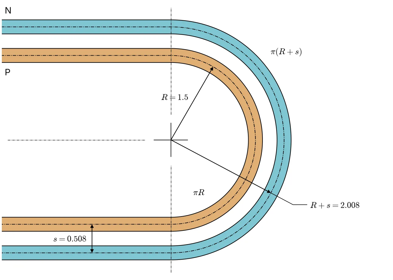
The bend on its own. The two arcs differ by π times the pitch, whatever the radius.
Test boards
Copperhead built one fixture and changed nothing but the tuning. Every board has the same stackup, the same launches and the same 12 mm legs.
C, D and F are the usual fix in three styles: two sparse excursions, a dense accordion of four and one broad trombone. On each, Copperhead solved the amplitude so that P and N come out exactly the same length, chamfered corners included. C far is C moved next to the launch. E is a control. It swings both traces out together, which adds delay to the pair and nothing to the difference between them. KiCad’s DRC passed every board before any of them went into the solver.
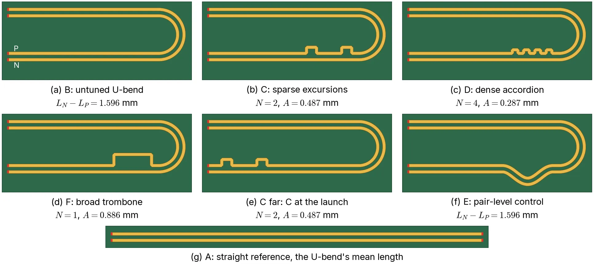
The boards as openEMS sees them. Every tuned board has P and N exactly equal in centreline length.
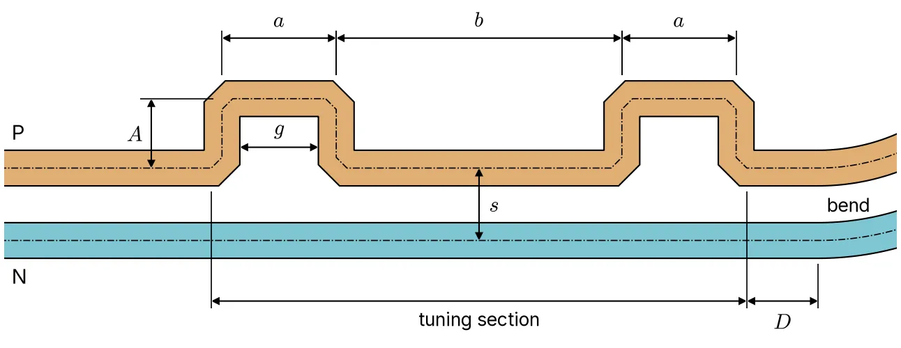
Board C. The serpentine makes P exactly as long as N, 30.308 mm each by the length report.
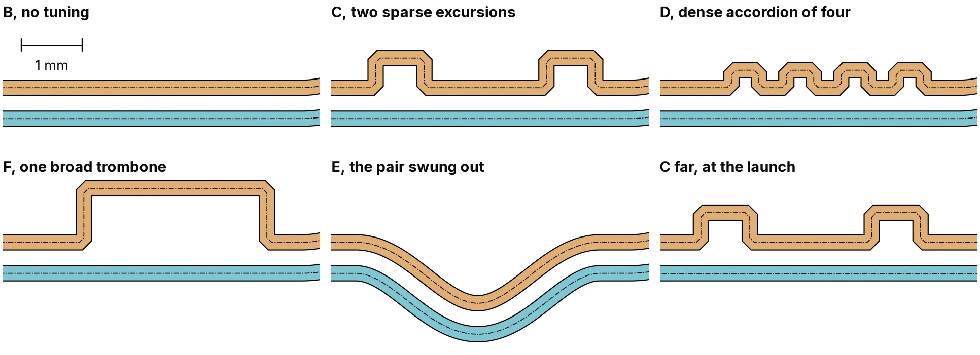
The tuning sections side by side, at one scale.
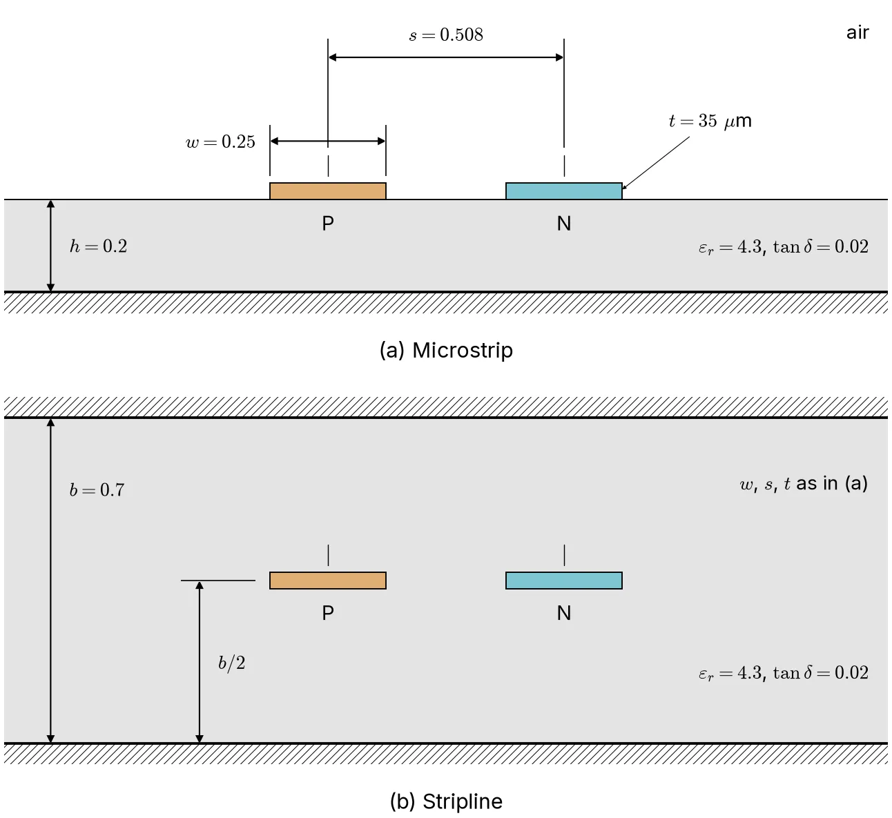
The two stackups, drawn at true scale. Everything below is microstrip until the stripline section.
Simulation
openEMS[2] solves Maxwell’s equations around the copper on a grid of cells. The board sits in a box: the copper on its dielectric, a perfect conductor underneath as the return plane and absorbing boundaries on the other five faces so the fields leave instead of reflecting back.
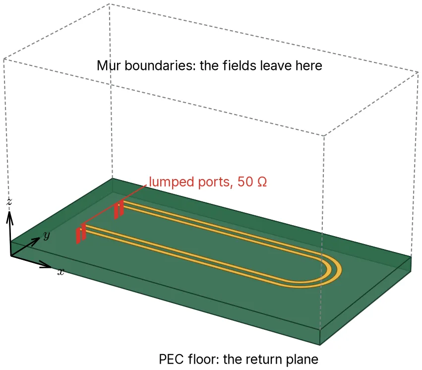
The model of board B. The height is drawn four times its true scale, or the slab would be a line.
Each run sends a pulse into one of the four ports, with the other three sitting there as 50 Ω loads[3]. Four runs give the full response of the board, its 4×4 S-matrix. scikit-rf[4] turns that into differential and common-mode terms, and from there into what a receiver sees for a 50 ps edge. All in, Copperhead ran 140 simulations.
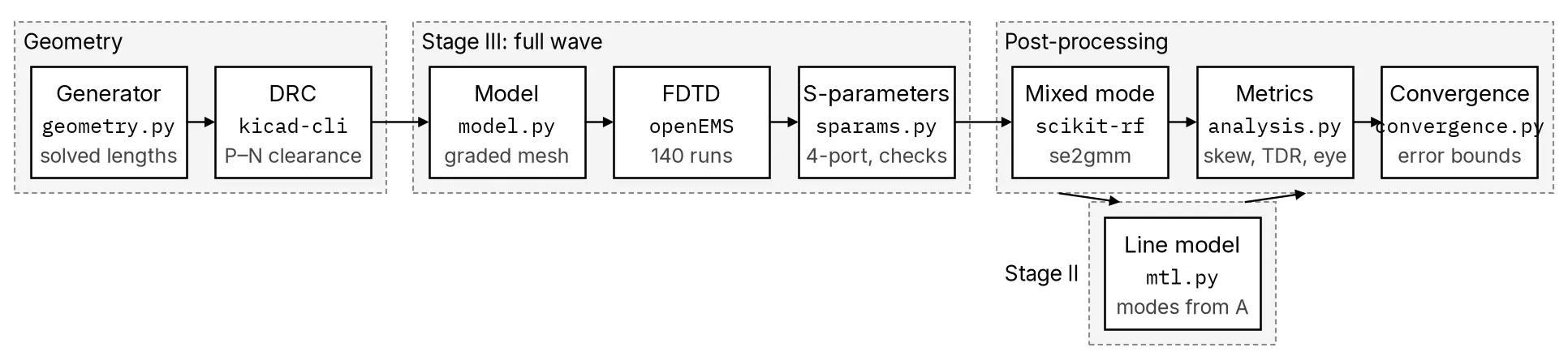
From copper to waveforms. The line model sits beside the full-wave results, calibrated on the straight board.
Mesh
The cells are 40 µm across over the copper and grow away from it, 1.24 million of them for a bent board. The 45-degree corner cuts come out as staircases at that size, which is the first thing to check.
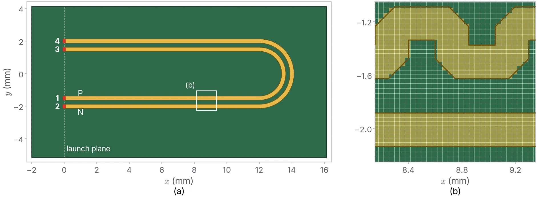
The domain as openEMS gets it, and the 40 µm mesh over board D’s corners.
So Copperhead solved the untuned bend, two of the tunings and the serpentines again on finer and coarser grids. On a 27 µm mesh the bend’s skew moves by only 0.02 ps. The bend’s skew carries ±0.05 ps, C’s ±0.3 ps and the dense accordion’s ±0.4 ps.
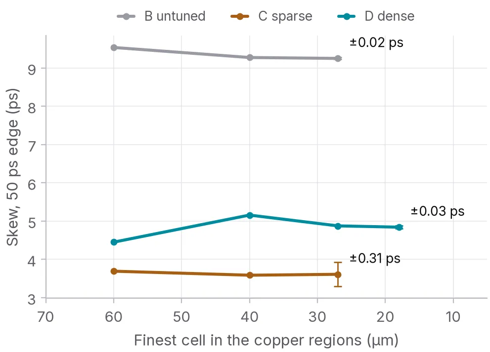
The skew on each mesh. The bend barely moves. The dense accordion needed a fourth mesh.
Skew after tuning
Every tuned board has P and N exactly the same length. Every one of them still lets P arrive first.
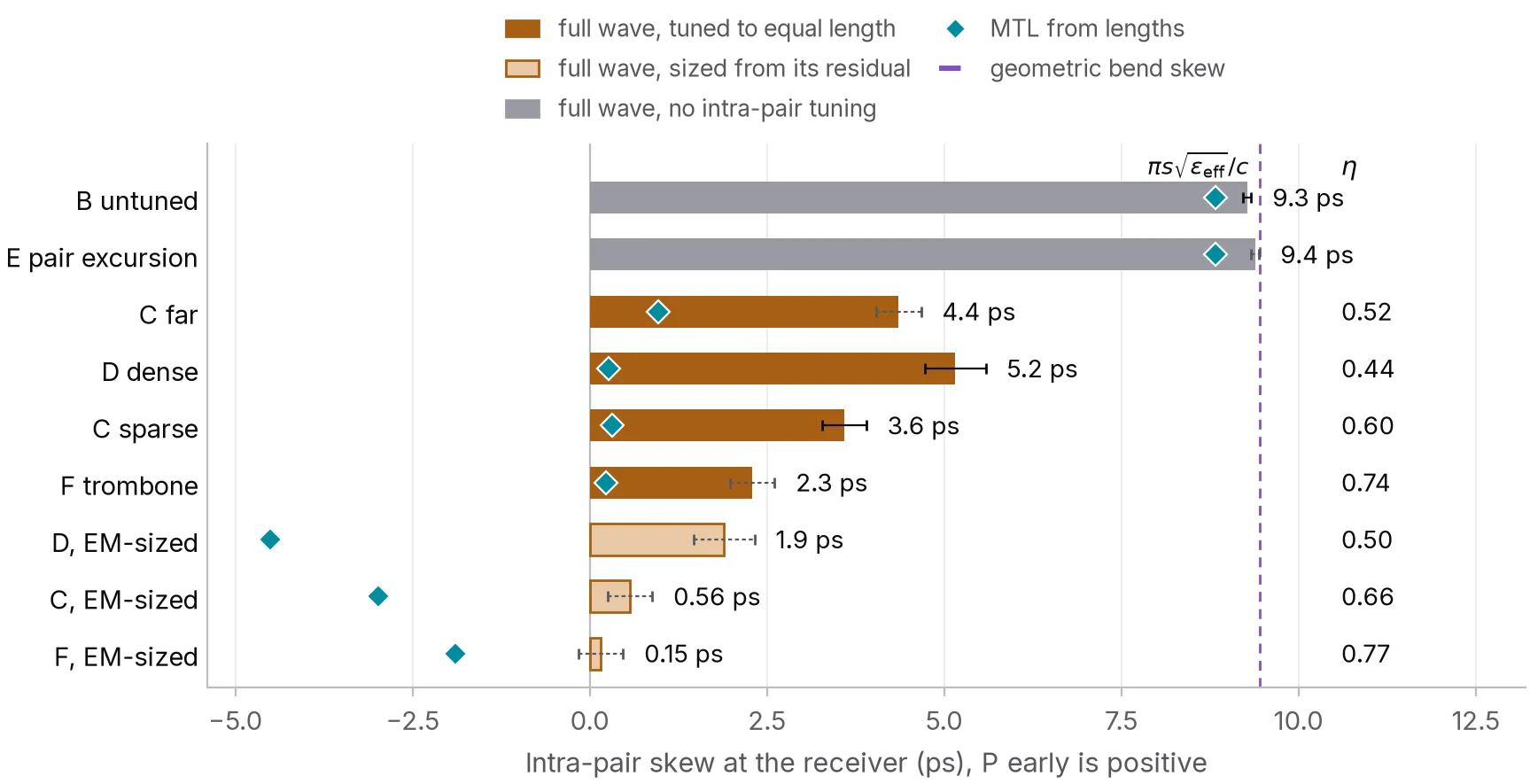
Skew at the receiver. The teal diamonds are what a model that only knows lengths predicts.
| Board | What it is | Skew left | Share of the bend’s skew removed |
|---|---|---|---|
| B | untuned bend | 9.3 ps | none |
| F | one broad trombone | 2.3 ps | 75 % |
| C | two sparse excursions | 3.6 ps | 61 % |
| C far | the same, at the launch | 4.4 ps | 53 % |
| D | dense accordion of four | 5.2 ps | 44 % |
| E | both traces swung out | 9.4 ps | none, by design |
The more excursions, the less of the skew came back: 75 % with one, 61 % with two and 44 % with four. It shows at the receiver too.
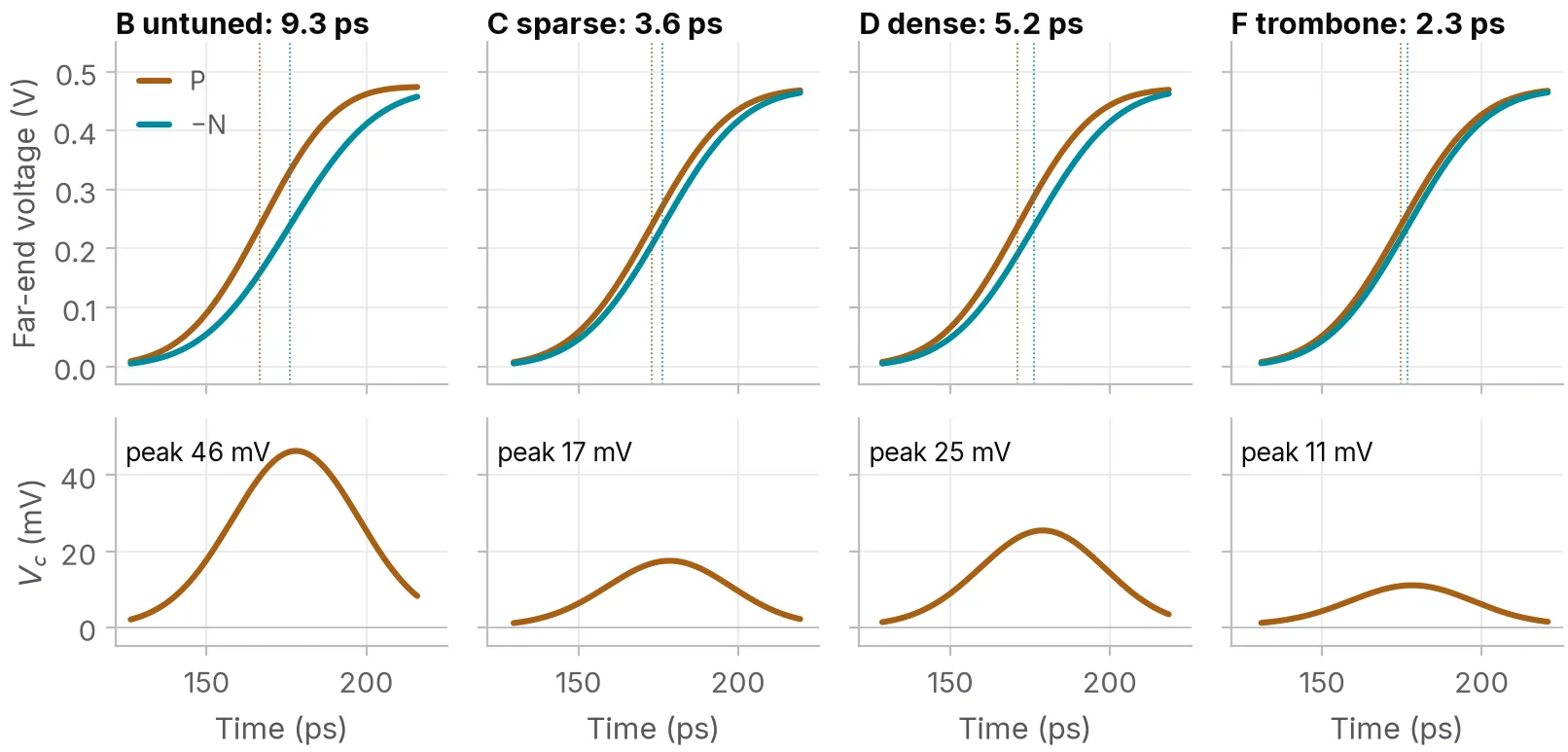
P still leads N on every board, and the common-mode pulse shrinks but never goes away.
Delay efficiency
The obvious suspect is the lengths. Copperhead built a transmission-line model of every board, calibrated on the solver’s own straight pair so its coupled lines are the solver’s coupled lines. It knows every length to the micrometre and predicts 0.2, 0.3 and 0.3 ps for F, C and D. Length isn’t what’s missing.
What the line model can’t see is the corners and the coupling between folds. To pull those apart Copperhead ran one more pair of boards. Each is a straight pair with 6 mm added to one trace in three excursions, once with the folds 1.0 mm apart and once at the 0.15 mm clearance rule. Same corners and same added length. They aren’t quite the same board, though. The tight one packs its folds into 2.15 mm against 6.40 mm, so P also spends less of its run away from N.
Call the delay a tuning actually adds, over what its length says it should add, its efficiency. The loose serpentine manages 0.84. Packed to the clearance rule it drops to 0.68, and it came out 16 to 24 points lower on every mesh. That fits the fold coupling Wu and Chao[5] and Rubin and Singh[6] found in single-ended meanders. It doesn’t prove it, because of those section lengths.
The loose serpentine’s own shortfall I’d put down to its corners, where the current cuts across the inside of each turn. That path is shorter than the centre line the length report measures. No board here changes the corners on their own, so that’s my best guess rather than a result.
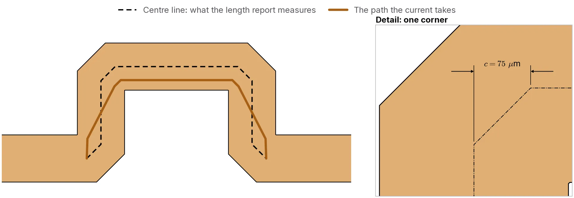
Why I think the corners cost delay. The current cuts the inside of each turn, so its path is shorter than the centre line.
In the bend fixes each excursion lost 1.6, 1.4 and 1.1 ps of the delay its length promised, for one, two and four excursions. The loss per excursion shrinks as the excursions get smaller, but not as fast as their number grows, so a fix built from lots of small excursions still does worst.
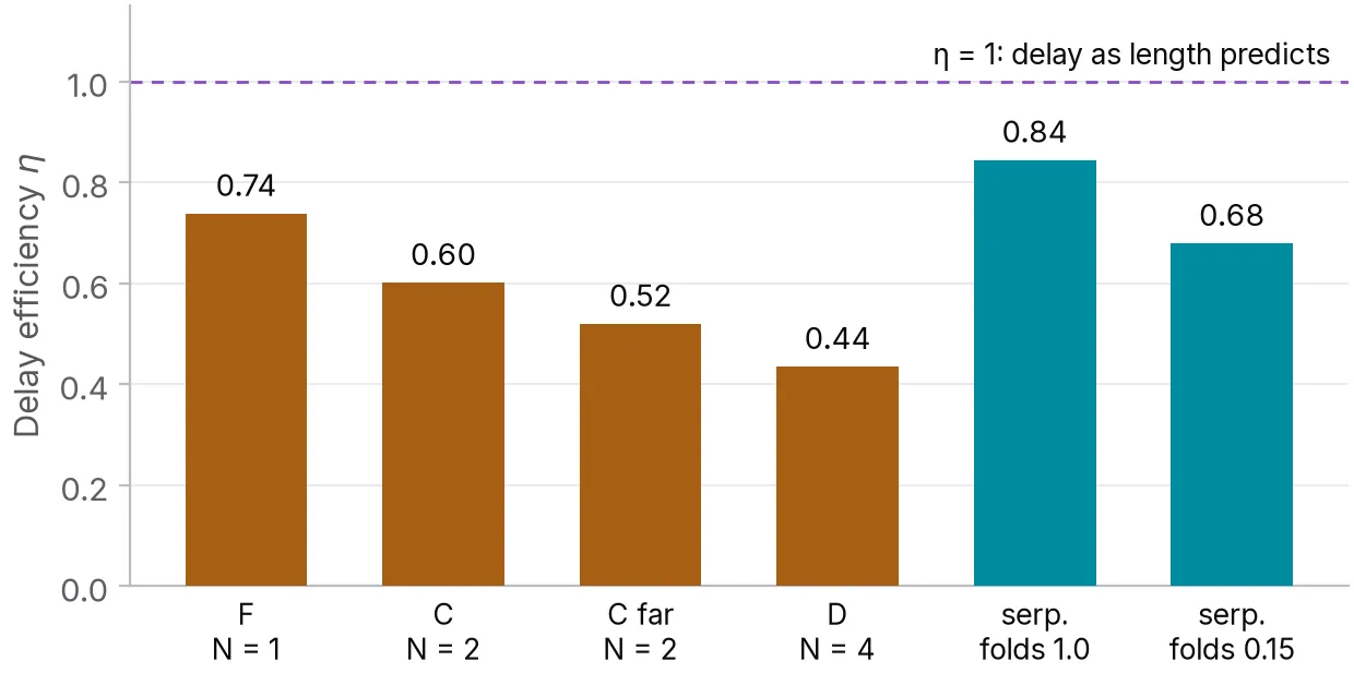
How much of its promised delay each tuning delivers.
Stripline
Microstrip runs its two modes at different speeds, so some of this could have been a microstrip quirk. Copperhead put the same copper between two planes and ran it again, on one mesh only.
It wasn’t. Geometry predicts the stripline bend to 0.6 % (10.97 ps against 11.04 ps). The tunings removed 81, 64 and 42 % of the skew. In microstrip they removed 75, 61 and 44 %.
Tight folds still cost 20 points. Copperhead had written into the first draft of its report that this penalty should shrink in stripline, because far-end coupling between parallel lines vanishes there. It doesn’t shrink. My best guess, which nothing here tests, is that neighbouring folds carry current in opposite directions. The coupling that shortcuts them would then be backward coupling, and stripline has plenty of that.
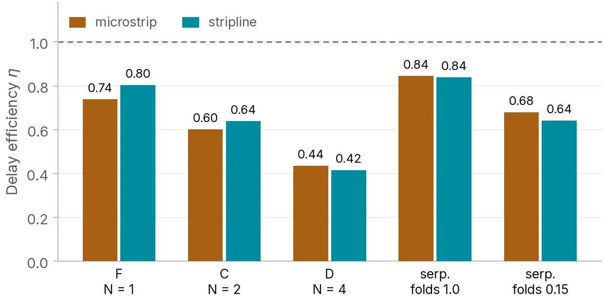
The same copper in microstrip and stripline, each against its own nominal velocity.
Tuning position
C far is the same tuning as C, moved next to the launch. Its skew at the receiver isn’t much worse (4.4 ps against 3.6 ps). Its mode conversion is. Between the tuning and the bend the pair carries skew the other way, and the two corrections drift out of phase as the frequency goes up. Read as a skew, C far’s grows from 4.1 ps at 5 GHz to 6.5 ps at 25 GHz while C’s stays flat. That’s one placement against another, not a sweep of the distance.
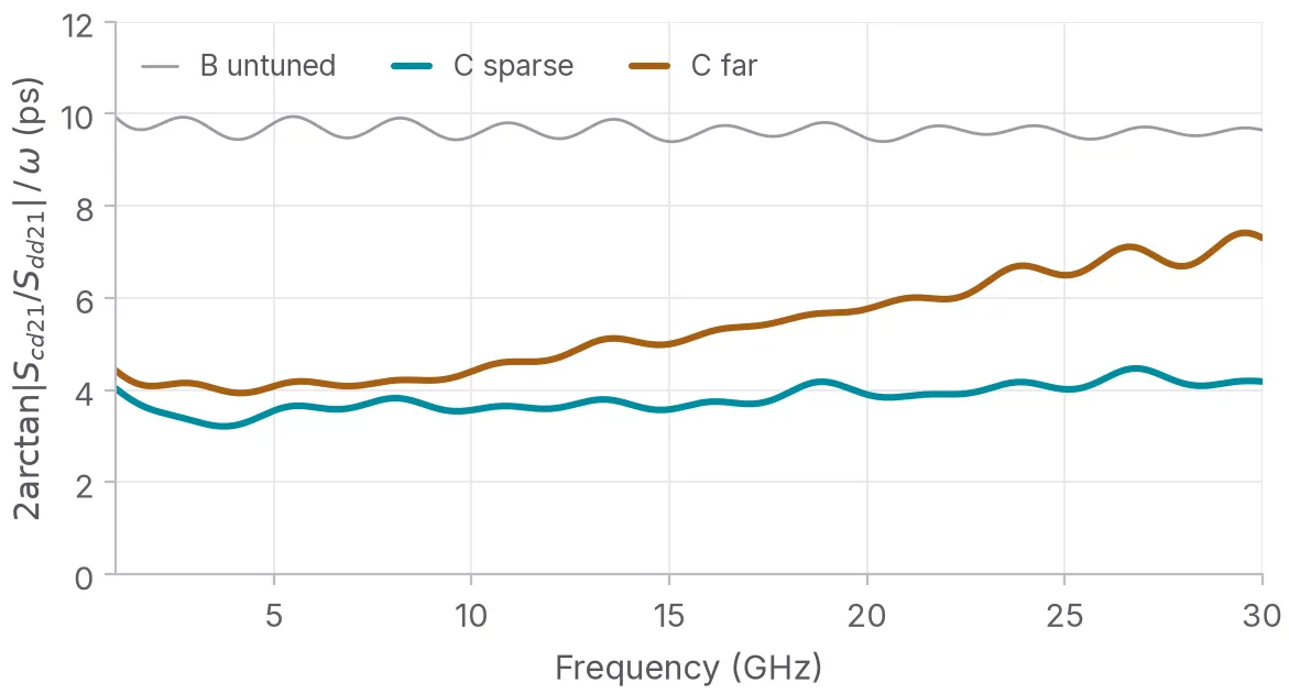
The same tuning next to the bend and at the launch, read as a skew at each frequency.
Impedance and return loss
The broad trombone removed the most skew. But its trace leaves its partner for 3 mm and the differential impedance there jumps to 114 Ω, against 107 Ω for the plain bend. Its return loss is the worst of the length-matched boards (−16.8 dB against −20.7 dB).
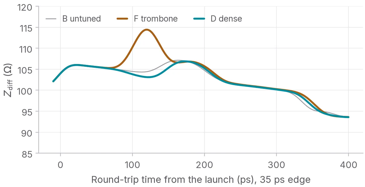
The trombone’s uncoupled stretch shows up as a bump on the TDR.
Eye and common mode
At 16 Gb/s with 35 ps edges, the untuned bend closes the eye from 92.9 % to 91.1 % of the swing. That’s small. The bigger effect is common mode, 13.6 % of the swing peak to peak at the receiver against 3.3 % for the trombone. A receiver with decent common-mode rejection won’t notice the timing. Whether the common mode becomes an emissions problem depends on the rest of the board, and none of this models that.
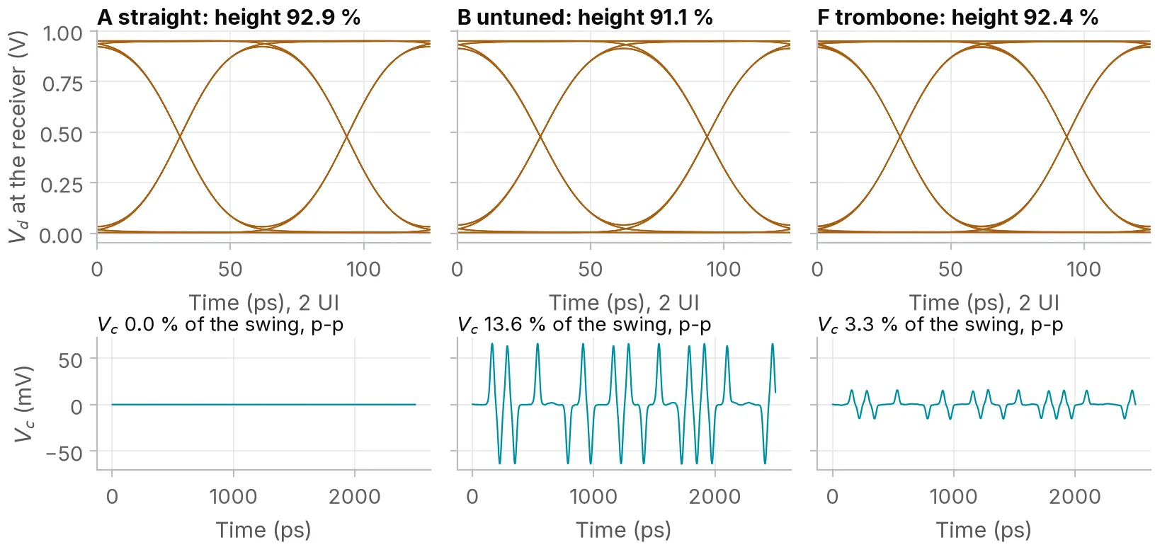
The eye barely moves. The common mode is where the skew shows.
Sizing from the residual
If each excursion loses a fixed amount, the fix is to put that amount back. Copperhead lengthened C, D and F by their own leftover skew, converted to length at the bend’s rate. By CAD measure P is now longer than N. The line model says all three overshoot: to -1.9 ps for F, -3.0 ps for C and -4.5 ps for D.
openEMS put F at 0.15 ps and C at 0.56 ps, so one iteration was enough for those two. Neither was rerun on other meshes, so the ±0.3 ps from C’s mesh check is a loan here, not a measurement. The dense accordion only came down to 1.9 ps. Each extra millimetre delivered 62 % of what it should have, against 83 % for C and 92 % for F. My guess is that stretching its tightly packed verticals tightens the coupling between them too.
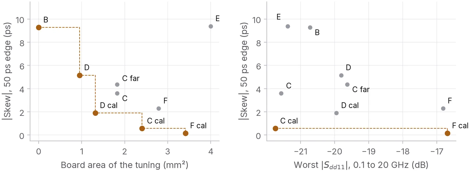
Skew against board area and against return loss. The points on the dashed line are the ones nothing else beats on both.
Design guidance
For edge-coupled pairs around this pitch, in microstrip or stripline:
- Trust geometry for the bend and not for the fix. Budget a few picoseconds of residual, or size the tuning from a field solve or a coupon.
- Use as few excursions as you can. The loss per excursion shrinks with its size, but not as fast as the count grows.
- Keep the folds apart. At the clearance rule they cost 16 to 24 points of efficiency.
- Tune next to the bend, not at the end of the route.
- Keep a broad excursion short or it’ll show up on the TDR.
- Swinging the whole pair out does nothing for skew within the pair.
Why Copperhead runs studies
It’s easy to build an AI for PCBs that’s judged by the rules it follows. DRC passes, the length report reads zero, done. On this bend that bar passes a board that still carries 5.2 ps of skew.
Copperhead works the other way round. It treats a rule as a claim to test, runs the study that tests it and keeps the result as a check with a number on it. This post is one of those studies from start to finish. Copperhead built the fixtures, ran the 140 solves, caught its own mistakes (below) and wrote the report.
The checks run on real designs through fang[8], Copperhead’s hardware kernel. A requirement that needs a simulation gets one. ngspice takes the circuits and Renode runs the firmware against the board it’s written for. A value that breaks a requirement never reaches the design. One that nothing has measured yet stays unknown instead of passing.
This study ran on its own scripts, beside fang rather than through it. fang can’t ask a field solver for skew yet, and the residual budget above is the first check I’d want it to run.
Errors during the study
The first runs never finished. openEMS stops once the energy in the model has decayed, and here it stalled well short of the target. Copperhead traced that to the DC content of the pulse, which leaves a static field behind that never decays. Every run now stops at a fixed 2 ns instead, after checking that the signals at the ports have fallen at least 98 dB.
The dense accordion wouldn’t converge. On three meshes its skew came out at 4.45, 5.16 and 4.88 ps. The honest bound on that is ±2.1 ps on a 5 ps result. Its 75 µm corner cuts are only a couple of cells wide. A fourth, finer mesh gave 4.84 ps and settled it at about 4.8 ps. The coarse mesh had been the outlier.
It also first scored the stripline boards against microstrip’s velocity, which made them look 17 % better than they are. That got caught because the loose stripline serpentine came out at 0.98, which didn’t fit anything else in the study.
Limitations
All of this is simulation. Nothing was built or measured. It’s one trace width and one pitch in one microstrip and one stripline stackup. The ports are lumped and the return planes perfect. The copper has no roughness.
Every full-wave number here comes from one solver, openEMS. The line model was calibrated on its runs, so the two agreeing isn’t an independent check. Nor are the mechanisms pinned down. The fold result is tangled up with section length, and the corners are a guess by elimination.
The report has a coupon plan for checking it on real boards. The first thing I’d want to see on a VNA is the dense accordion leaving 5.2 ps where the length report says zero.
Full report
Copperhead wrote the report and drew every figure in this post. It runs to 14 pages with the method, the mesh checks, the related work and the coupon plan. Copperhead checked each of its 26 references against Crossref or its source page[9]. The scripts, the S-parameter files and the raw solver runs are in the study’s repository. A script fills in every number in this post from those files.
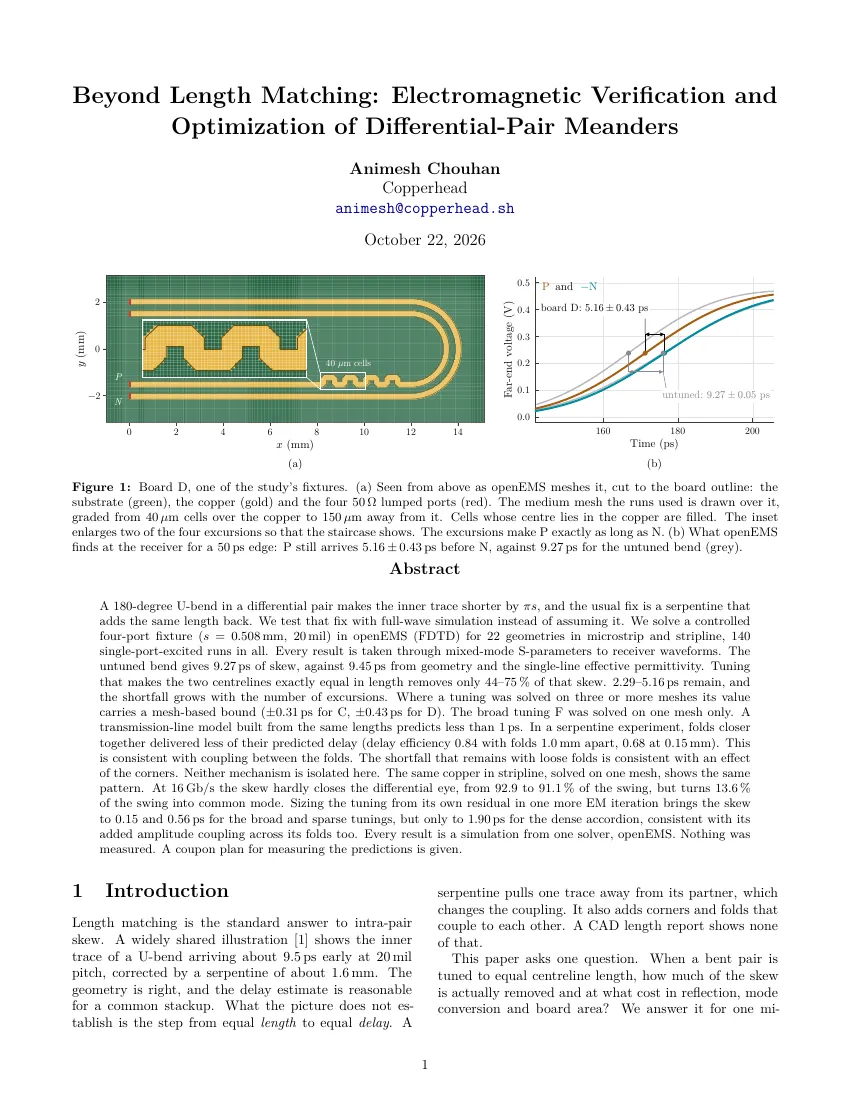
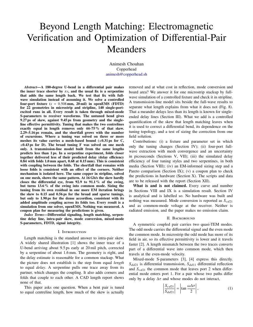
The report and the same text in IEEE format. Each opens the PDF.
| Document | Pages | File |
|---|---|---|
| Beyond Length Matching, report | 14 | PDF, 0.8 MB |
| Beyond Length Matching, IEEE format | 13 | PDF, 0.8 MB |
References
Each entry says which claim in the text it carries. Web sources were read on 19 October 2026.
-
@CorneliusWrites, post on X.
https://x.com/CorneliusWrites/status/2110776676795953595
The 9.5 ps and 1.6 mm this post starts from. The post wouldn’t load for re-checking on 19 October 2026. -
openEMS Project, Introduction.
https://docs.openems.de/en/latest/intro.html
The field solver, an equivalent-circuit FDTD code. The runs used version v0.37.0-rc3-31-g6761a36. -
openEMS Project, Ports.
https://docs.openems.de/en/latest/concepts/ports.html
One excited port per run with the rest passive, which is how the 4×4 matrix is built. -
scikit-rf, Network.se2gmm.
https://scikit-rf.readthedocs.io/en/latest/api/generated/skrf.network.Network.se2gmm.html
The conversion to differential and common-mode terms. Its port order was checked against the source of scikit-rf 2.2.0 rather than the rendered docs. -
R.-B. Wu and F.-L. Chao, Laddering wave in serpentine delay line, IEEE Trans. Compon., Packag., Manuf. Technol. B, vol. 18, no. 4, 1995.
https://doi.org/10.1109/96.475270
Coupling between the segments of a serpentine shortens its delay. -
B. J. Rubin and B. Singh, Study of meander line delay in circuit boards, IEEE Transactions on Microwave Theory and Techniques, vol. 48, no. 9, 2000.
https://doi.org/10.1109/22.868994
The same effect in meanders, modelled and measured. -
E. Hammerstad and O. Jensen, Accurate models for microstrip computer-aided design, 1980 IEEE MTT-S International Microwave Symposium Digest.
https://doi.org/10.1109/MWSYM.1980.1124303
The single-line ε_eff of 3.15 behind the 9.45 ps. -
Copperhead, fang.
https://github.com/copperheadhq/fang
The hardware kernel and its verification questions: ngspice and Xyce for circuits, Renode for firmware, KiCad’s ERC and Touchstone files for RF. -
Beyond Length Matching: Electromagnetic Verification and Optimization of Differential-Pair Meanders, 14 pages.
/research/diffpair-meanders.pdf
Every number in this post with its method, its mesh checks and the limitations.
Cite this article
@misc{chouhan2026diffpairmeanders,
  author       = {Chouhan, Animesh},
  title        = {{Simulating serpentine length matching on a bent differential pair}},
  howpublished = {Copperhead research},
  year         = {2026},
  month        = oct,
  url          = {https://copperhead.sh/research/diffpair-meanders/},
  note         = {Code: \url{https://github.com/copperheadhq/copperhead-research/tree/main/diffpair-meanders}}
}Chouhan, A. (2026). Simulating serpentine length matching on a bent differential pair. Copperhead research. https://copperhead.sh/research/diffpair-meanders/